In our recent video about O-rings, we featured some FEA animations of an O-ring being installed in a gland, and then responding to applied pressure. We have received a few questions about how this simulation was performed, so we thought we’d make this blog post to expand on that a bit.
Before diving into the details, it’s important to mention that there actually aren’t a lot of cases that justify a full-blown hyperelastic FEA of an O-ring. There is quite a bit of empirical data available that will allow you to avoid having to simulate the O-ring itself. For example, we mention in the video that face seals require quite a bit of clamping force to compress evenly. If you were designing an enclosure with a face seal, and wanted to determine the deformations in the mating halves due to the O-ring compression force, you wouldn’t need to simulate the O-ring. You could use Figures 2-4 through 2-8 in the Parker O-Ring Handbook to determine the compression force per unit length for your particular cross section, hardness, and squeeze, and then just apply this force to each of the components directly. That is exactly what we did to generate the plots in the video starting at 2:20.
So, consider the text that follows more of an introduction to setting up a hyperelastic FEA study. This type of study is useful for analyzing more complicated designs like metal spring-energized (MSE) seals, vee-packing, wipers, and bellows. All of these components (as well as O-rings) are comprised of elastomeric compounds, which is a class of materials that can withstand tremendous strain (often greater than 100%) without breaking.
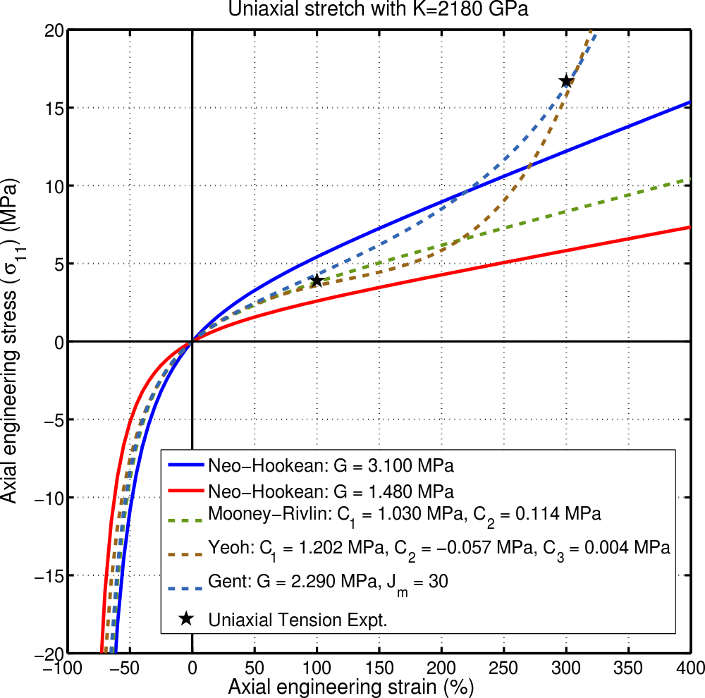
Simulating these types of materials with FEA requires a hyperelastic material model like Mooney-Rivlin, Neo-Hookean, or Ogden. The models are generated from material test data, and while you may be able to find the data in academic literature, you will likely need to pay a polymer testing company to generate it for you. The particular model to use depends on the behavior of the material and the test data that is available. For rubbers, Ogden (2nd-order or 3rd-order) is typically preferred.
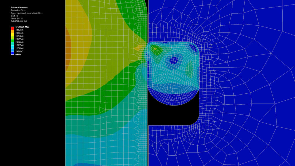
For the O-ring study that we showed in the video, the geometry of the gland was modeled according to the static O-ring design tables in the Parker handbook. The O-ring itself was also modeled in its undeformed state. An axisymmetric study was used to reduce the problem size.
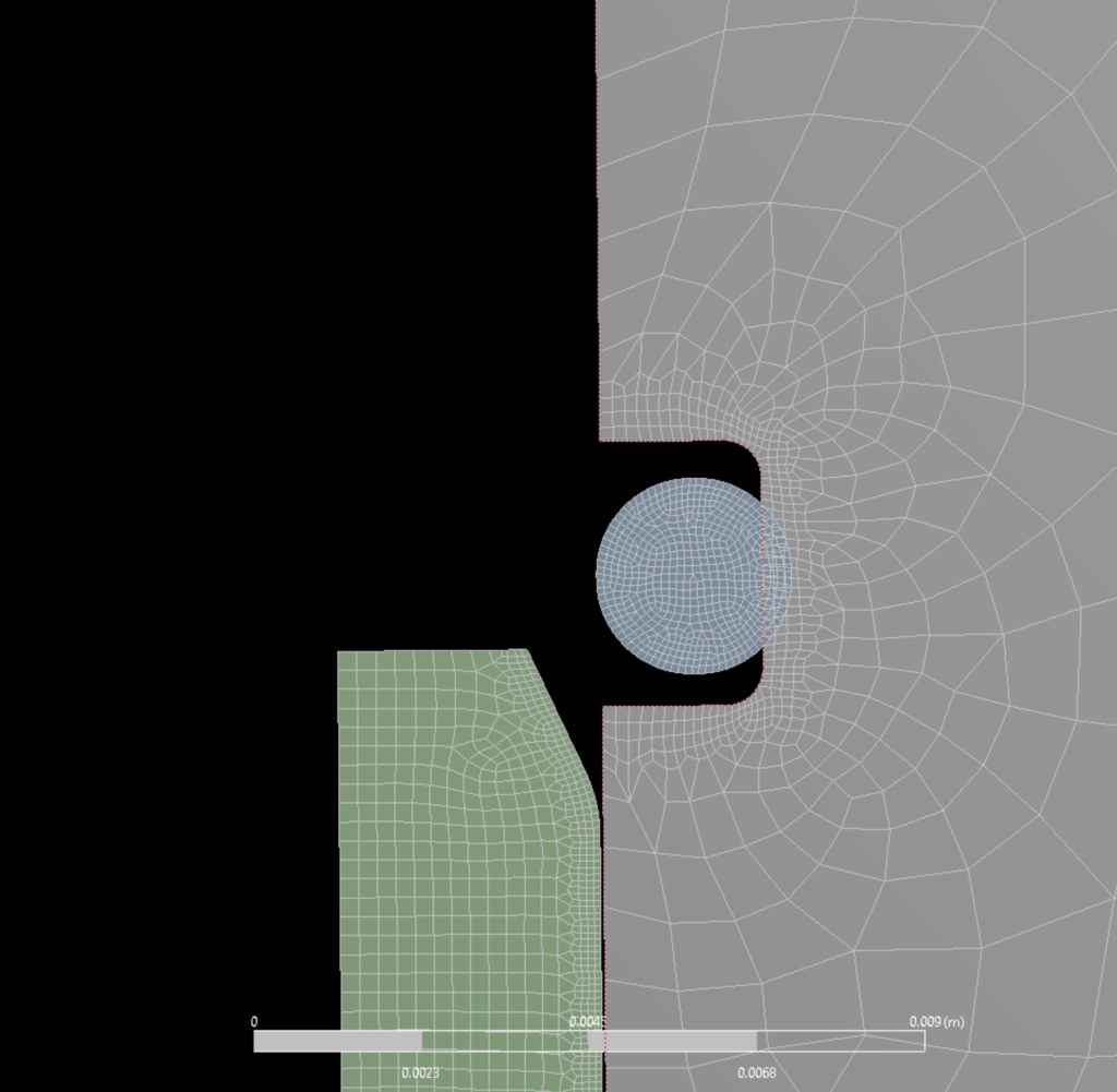
Contact sets were created between the O-ring and the groove, and the O-ring and the piston. It is important to specify a coefficient of friction for these contact sets to help the solution converge.
The simulation is performed in three steps: 1) stretch the O-ring into the gland, 2) install the piston to squeeze the O-ring, and 3) apply the pressure. The stretch step simply resolves the contact set between the groove and the O-ring, and no boundary conditions or loads are applied. In the squeeze step, a displacement boundary condition is applied to the piston (to force it to stab into the O-ring) and the contact sets work to eliminate the interference as this happens.
Applying the pressure load is a bit more complicated. We mentioned in the video that in seals, the fluid only penetrates to the point where the contact stress is equal to the fluid pressure. To simulate this effect in FEA, you need to use a special load called “pressure penetration.” This is a load that is also linked to a contact set, and the solver determines the area over which to apply a pressure load by iteratively comparing the contact stress to the fluid pressure. In ABAQUS, pressure penetration is available through the ABAQUS/CAE graphical interface, but as of ANSYS 2019, you must use ADPL. Hence, if you have a choice between the two, I’d recommend ABAQUS for this type of problem.
If you’re interested in performing a similar study yourself, be sure to take a look at the resources we’ve linked below. There are some sample material parameters, as well as a tutorial for setting up the ADPL commands for pressure penetration in ANSYS.
Resources
- B. Liao, B. Sun, M. Yan, Y. Ren, W. Zhang, and K. Zhou, “Time-Variant Reliability Analysis for Rubber O-Ring Seal Considering Both Material Degradation and Random Load,” Materials, Oct. 2017.
- Values for a 3rd-order Ogden model of a 70-durometer compound are given on page 15.MSC Software, “Nonlinear Finite Element Analysis of Elastomers,” Nonlinear Finite Element Analysis of Elastomers.
- Parker Hannifin Corporation, Parker O-Ring Handbook.
- Ansys Inc, Applying Fluid Pressure Penetration Loads.
- Kelly, “Isotropic Hyperelasticity“.
- H. Wong, L. Zeng, “Seal Evaluation Using ANSYS WorkBench,” Automotive Simulation World Congress, 2012.
- Ansys Inc, Fluid Pressure Penetration.
- Detailed tutorial showing how to apply pressure penetration loads using APDL commands within ANSYS Mechanical.
Great article. Concise, informative and to-the-point!
Thanks for it.